Once I built the filters, I started to build the QRPLabs relay switch for automatically select up to 5 different filters by my raspberry.
The board is designed to fit with Ultimate3/3S transmitter, but can be interface to other systems adding simple BJT switches, as suggested on QRPLabs website.
I put the 5 transistors, the bias resistors and striplines connector on a prototype PCB having the same dimensions of the switches board, and is connected below it using the headers provided in the relay kit.
For RF input, I used a short piece of RG142 coax cable, terminated with an SMA male to be plugged on the VNA for initial characterization. Later, I replaced the SMA with a 2pins female stripline contact which can be plugged directly on the Raspy headers. On the other side, I soldered the coax directly to the PCB pins.
Here below some pictures:
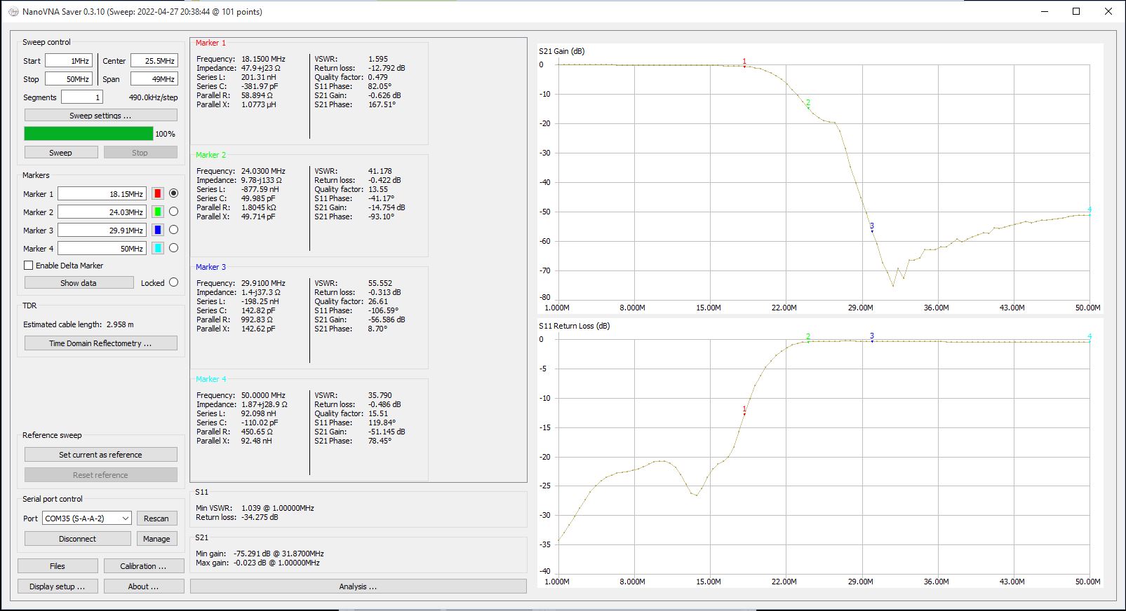
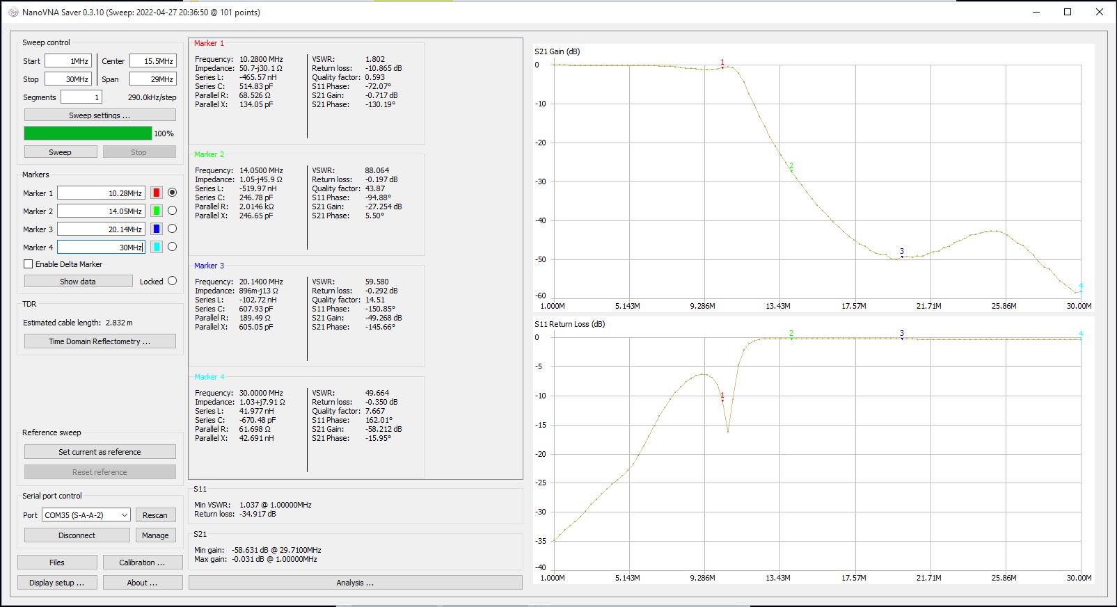
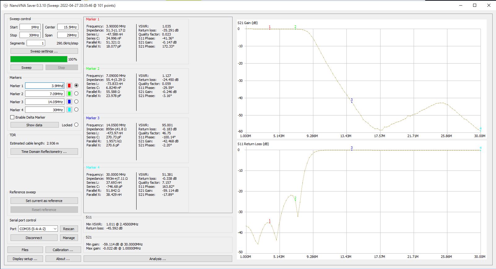
I repeated all the filter measurements previously done on the filters connected one by one to the VNA by means of PH2LB fixture, but this time using the relay board. Here below the results:
The in-band attenuation is very similar toe the previous results, so it demonstrates that the relay board introduces a very small attenuation.
The main difference is the out-of-band attenuation , which has a strange trend (decreases and increases again with frequency).
I don’t know why the isolation is worst than the expected. This could be due to some coupling effect on the PCB. I’m going to share the results on QRPLabs forum for understanding better.
If I come to some conclusion, I’ll write down here!
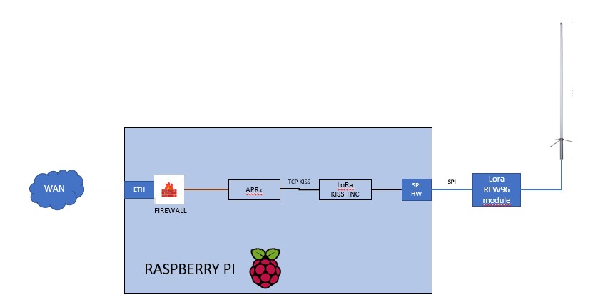
When I started experimenting with LoRa, I wasn’t sure it would thrill me (it did!), so I was looking for a minimal cost setup, without investing too much in hardware. In studying the possible solutions, I stumbled upon the Austrian LoRa OM site and found that there were schematics available for a very compact tracker that could also act as a Gateway. However, the funniest idea was to integrate the Lora with the 144.800VHF network already present on my digi / I-gate of which I am sysop, to create a cross-band and cross-protocol digipeater between VHF FSK1200baud and UHF LoRa. Still on the Austrians’ website, I discovered that there is a Software Modem that was created to interface with aprx, the software I have been using on my digipeater for over 10 years and which still remains one of the most versatile in the APRS field.
This configuration requires that the software that implements the TNC (in this case RPi-LoRA-KISS-TNC) and the software that takes charge of the packets to and from the TNC and then manages them according to the APRS protocol (in this case aprx) are connected to each other through the KISS protocol encapsulated in TCP-IP.
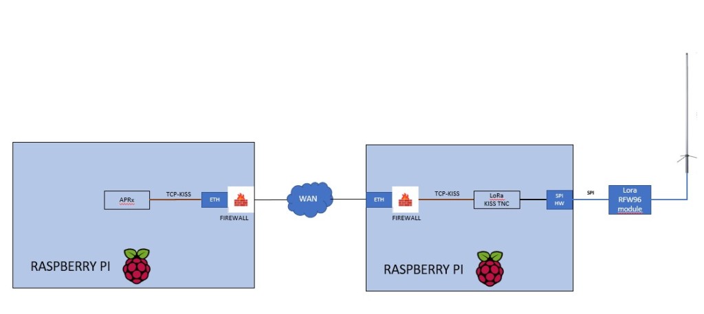
Using a tcp-ip link, the possible scenarios are the following:
Aprx (or equivalent) and RPi-LoRa-KISS-TNC installaed on the same host and linked by loopback 127.0.0.1:
Aprx (or equivalent) and RPi-LoRa-KISS-TNC installed on different hosts and maybe even distant from each other (interesting configuration):
My case is the first, that is software that run on the same raspberry, so a port of this type must be declared in the aprx.conf file:
The port must obviously be the same as the one declared in config.py of the RPi-LoRa-KISS-TNC.
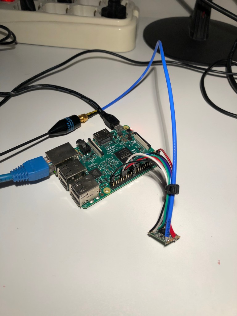
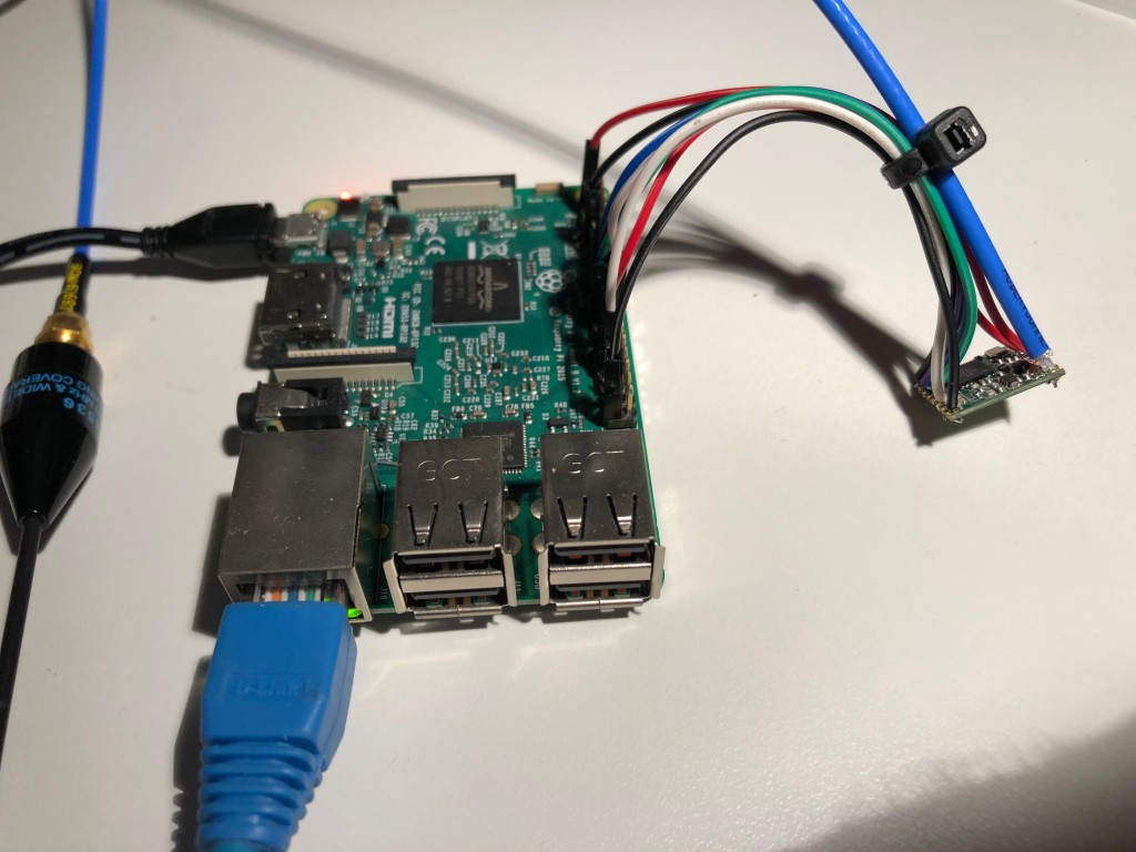
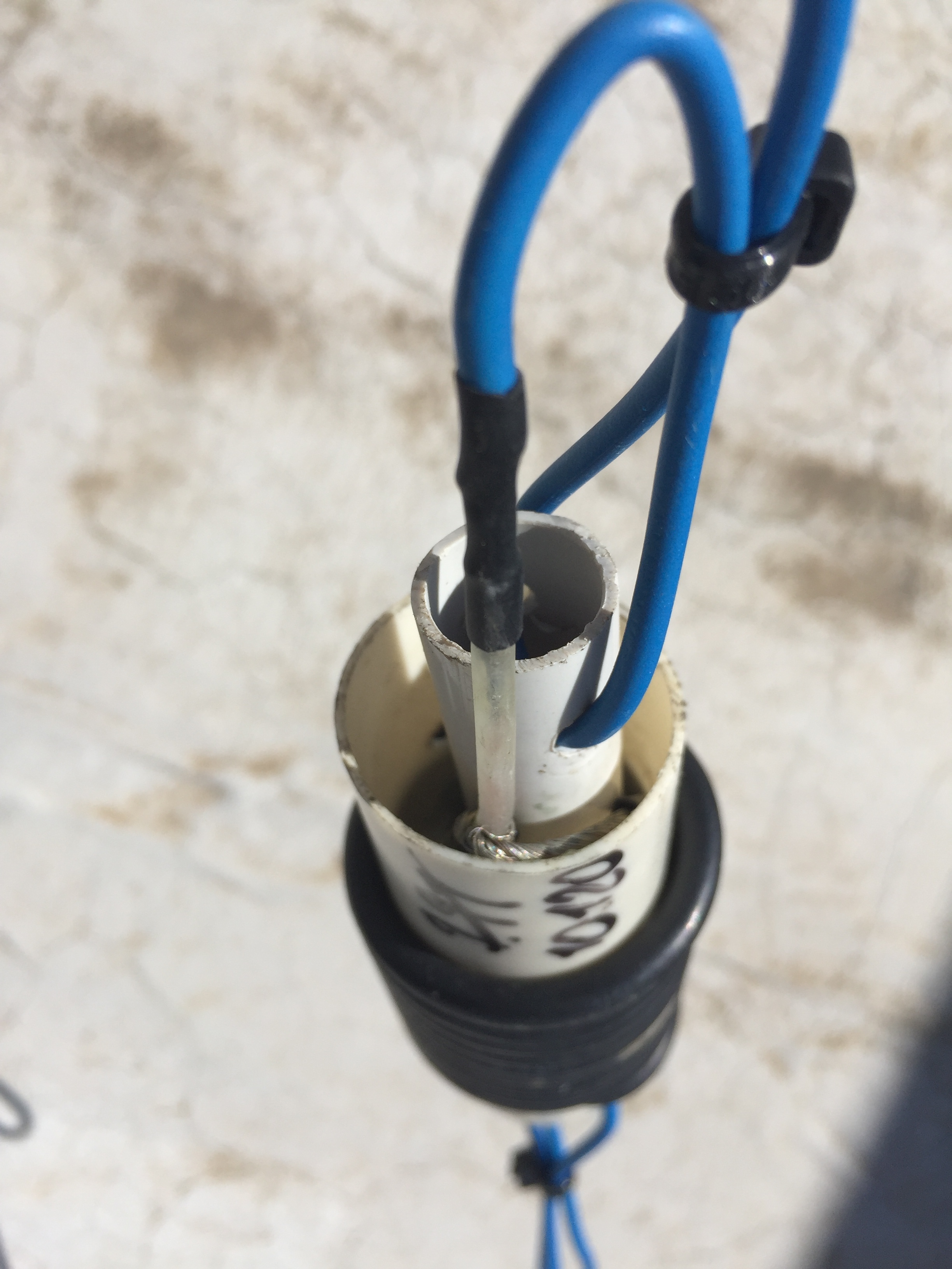
I therefore decide to take this path and order an RFW96 module from aliexpress, to connect it to the raapberry SPI as indicated on the software installation how-to. After about 3 weeks, a couple of LoRa modules arrive from China. Unfortunately the Lora module has a very narrow pitch pinout, incompatible with the 2.54mm standard, so the ideal would be to use an adapter PCB. I ask the “IOT4PI” group for the PCB that was created for this purpose, but they tell me that they no longer have it available, so I decide to connect it to the raspy in a flying way. I proceed with some simple pieces of prototype jumpers (female square pins) and I can wire the LoRa module towards the raspberry following the Austrian scheme. I manage to solder a thin Teflon cable on the pads of the antenna output, and at the other end of the coax cable I fix a flying SMA. In the photo below the final result.
Both the software and the hardware worked immediately and I started conducting the first tests that immediately showed me the potential of this protocol. During the first period of experimentation I also had the opportunity to find and solve some small bugs on the software and to start communicating constructively with TOM, the author of the Software.
After this first phase, I came into contact with the Italian group SARIMESH, very active in the Lora experimentation, which has as its reference the very kind OM Michele I8FUC.
I learned that Sarimesh set their software to be compatible with both that of the Austrian group (baptizing it “OE_style”) and with the standard ax25. The idea is more than acceptable, because we should always avoid proprietary protocols and stick to the standard ones. However it must always be considered that the speed of the Lora is low and the ax25 produces a slight data overhead, so this trade-off is always in question.
From the need to maintain the ax25, the idea of expanding the RPi-LoRa-KISS-TNC was born.
During the first stages of debugging, I had already had the opportunity to understand the structure of the code written entirely in python and luckily Tom had also added some comments that made my work easier. Editing was easy enough and only took me a few hours of time.
The discrimination of the received packet is based on a packet header which was chosen by the Austrian OMs as their standard identifier, and consists of the 3 bytes “0x3C 0xFF 0x01”. Once I have received the packet, I check for the presence of this header. If present, then it is an “OE_Style” package to be processed with the functions already present in the code, otherwise it is a standard AX25 package.
To learn more about the structure of a standard AX25 frame, in addition to reading the protocol, I also recommend reading this excellent article, which also has a simulator that builds the frame in real time starting from editable fields.
Here below, a typical structure of a kiss frame is reported:
In case of ax25 package, the job is very simple: you take the package and encapsulate it in KISS.
KISS is a very simple protocol. In our case, what I do is simply:
Add at the beginning and at the end a byte “0xC0” of Frame start and Frame End;
After the first Start byte, I add a “0x00” byte. This packet is divided into two nibbles: the most significant is the port number (in the case of a single TNC it is “0”), while the least significant is the command. Again from the protocol, we see that the command “0” is the one that must always precede a data frame when it is passed from the tnc to the user. So basically this byte is always “0x00”.
Vice versa, the packet to be transmitted in Lora is received by the software, de-encapsulated by the kiss (thus eliminating the delimiters and the “0x00” byte described above) and transmitted as it is via LoRa RF.
While making these changes, I have also implemented these improvements:
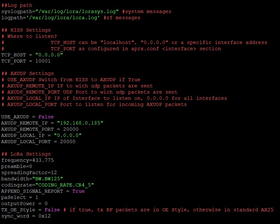
Brought all the Lora configuration parameters (sync word, bandwidth, spread factor, preamble lenght, power, etc ..) into the config.py configuration file. Before, the parameters were hidden inside the code and it was a bit difficult to find them without a minimum of programming skills.
Added a printout of all these parameters at the start of the software, which is always useful to remind the user in what conditions the tnc was started.
Added printouts of the source call and the destination call of the standard ax25 packages, using the functions already present in the code.
Added log files to log both RF packets and system messages.
The configuration file is commented as much as possible to avoid user errors. A note on the “TX_OE_Style” parameter: it is a Boolean (therefore it can only assume a True / False status) which determines the transmission format. While in reception the TNC accepts both OE / ax25 formats, obviously in transmission we must necessarily choose one of the two, and this is done with this parameter.
Another obvious consideration: the parameters of the LoRa protocol (sync word, spread factor, etc.) will be the same in the case of OE_Style or ax25 packets, and it is not possible to differentiate them because the LoRa module only accepts a set of parameters to be initialized.
Here below, an example of cofig file:
You must also be careful to declare a valid path for the log files, and with the right write permissions, otherwise the software will fail on startup.
Below you will find some example screens in the various operating phases.
The following is the start-up screen with all the initialization parameters.Note the string announcing the successful connection between RPi-KISS-TNC and the client software, in this case APRX.
The following, is an ax25 packet receiver via KISS-TCP and transmitted by LoRa interface:
Here below, a OE_style packet riceived by LoRa channel and passed to aprx via KISS-TCP:
The previous packet (OE_style) received by aprx via KISS-TCP:
Packet received via LoRa in ax25 fromat and passed to aprx via KISS-TCP:
Here below, you can see as the austrian tracker is correctly receiving a beacon originated by aprx , passet to RPi-LoRa-KISS-TNC by KISS-TCP and transmitted o LoRa channel:
So far the software is behaving stably and has never crashed. Obviously anyone who wants to try it, test it and possibly contribute to the development with code modification or suggestions, is welcome!
The source is available on my github. The installation is described in the INSTALL.md file and is fairly straightforward. It plans to download, using the “git clone” command, the content from github to a local folder of the raspberry, and to download the python libraries of the LoRa module in a subfolder.
ATTENTION !: install.md says to go and modify the content of the pySX127x / SX127x / board_config.py file and change the mapping of one of the GP / IO pins of the raspberry dedicated to interfacing with the LoRa module :
This modification is in line with the connections provided in the wiring diagram, but there is nothing to prevent the original mapping from being changed, always consistently with the diagram, as long as the GP/IO lines are free and not used by other processes.
Take care also of the log files, which can become big. Configure logrotate for a correct storing strategy.
The log files are very useful because they store also corrupted packets which are not passed to and from aprx, but sometimes contain useful information.
I want to thank the original author, Tom OE9TKH who was the first creatorof the Software I expanded.
Quando ho iniziato la mia sperimentazione in LoRa, non ero sicuro che mi avrebbe entusiasmato (invece è successo!), quindi cercavo un setup a costo minimo, senza investire troppo sul Hardware. Nello studio delle possibili soluzioni, mi sono imbattuto sul sito degli OM austriaci e ho scoperto che erano disponibili gli schemi per un tracker molto compatto che poteva fare anche da Gateway. Tuttavia, l’idea più divertente era quella di integrare il Lora con la rete 144.800VHF già presente sul mio digi/I-gate di cui sono sysop, per realizzare un digipeater cross-band e cross-protocol tra VHF FSK1200baud e UHF LoRa. Sempre sul sito degli austriaci, ho scoperto che esiste un Software Modem che nasce proprio per interfacciarsi con aprx, il software che uso sul mio digipeater da oltre 10anni e che tutt’ora rimane uno dei più versatili in ambito APRS.
Questa configurazione prevede che il software che implementa il TNC (in questo caso RPi-LoRA-KISS-TNC) e il software che prende in carico i pacchetti da e verso il TNC per poi gestirli secondo il protocollo APRS (in questo caso aprx) siano connessi tra di loro attraverso il protocollo KISS incapsulato in TCP-IP.
Sfruttando un link tcp-ip, gli scenari possibili sono i seguenti:
Aprx (o equivalente) e RPi-LoRa-KISS-TNC installati sullo stesso host e quindi collegati in loopback su indirizzo 127.0.0.1 :
Aprx (o equivalente) e RPi-LoRa-KISS-TNC installati su host differenti e magari anche distanti tra loro (configurazione interessante):
Il mio caso è il primo, ovvero software che girano sullo stesso raspberry, quindi nel file aprx.conf deve essere dichiarata una porta di questo tipo:
La porta deve essere ovviamente la stessa di quella dichiarata in config.py del RPi-LoRa-KISS-TNC.
Decido quindi di intraprendere questa strada e ordino un modulo RFW96 da aliexpress, per collegarlo alla SPI del raapberry così come indicato sul how-to di installazione del software. Dopo circa 3 settimane mi arriva dalla Cina una coppia di moduli LoRa. Purtroppo il modulino Lora ha un pinout a passo molto stretto, incompatible con lo standard 2,54mm, quindi l’ideale sarebbe usare un PCB di adattamento. Chiedo disponibilità al gruppo “IOT4PI” del PCB che nasce proprio per questo scopo, ma midicono che non ne hanno più a disposizione, quindi decido di collegarlo al raspy in maniera volante. Procedo con dei semplici spezzoni di ponticelli da prototipo (femmine pin quadri) e riesco a cablare il modulino LoRa verso il raspberry seguendo lo schema austriaco. Riesco a saldare un sottile cavetto in teflon sui pad delL’uscita d’antenna, e all’altro capo del cavetto coax saldo un sma volante. Nella foto sottostante il risultato finale.
Sia il software che l’hardware hanno funzionato da subito e ho iniziato a condurre le prime prove che mi hanno subito mostrato le potenzialità di questo protocollo. Durante il primo periodo di sperimentazione ho anche avuto modo di trovare e risolvere qualche piccolo bug sul software e di iniziare a comunicare costruttivamente con TOM , l’autore del Software. Dopo questa prima fase, sono entrato in contatto col gruppo italiano SARIMESH, molto attivo nella sperimentazione Lora, che ha come riferimento il gentilissimo Michele I8FUC. Ho appreso che loro avevano impostato il loro software per essere compatibile sia con quello del gruppo austriaco (battezzandolo “OE_style”) che con lo standard ax25. L’idea è pià che condivisibile, perchè bisognerebbe sempre evitare protocolli proprietari e mantenersi su quelli standard. Tuttavia bisogna sempre considerare che la velocità del Lora è bassa e l’ax25 produce un leggero overhead di dati , quindi questo compromesso è sempre messo in discussione. Dalla necessità di mantenere l’ax25, nasce l’idea di espandere RPi-LoRa-KISS-TNC. Durante le prime fasi di debug, avevo già avuto modo di capire la struttura del codice scritto totalmente in python e per fortuna Tom aveva anche aggiunto qualche commento che mi ha facilitato il lavoro. La modifica è stata abbastanza facile e mi ha portato via solo qualche ora di tempo. La discriminazione del pacchetto ricevuto si basa su un header del pacchetto che è stato scelto dagli OM austriaci proprio come identificativo del loro standard, e consiste nei 3 byte “0x3C 0xFF 0x01”. Una volta ricevuto il pacchetto, verifico la presenza di questo header. Se è presente, allora trattasi di pacchetto “OE_Style” da procesare con le funzioni già presenti nel codice,altrimenti trattasi di pacchetto standard AX25.
Per approfondire la struttura di un frame standard AX25 consiglio, oltre alla lettura del protocollo, anche la lettura di questo ottimo articolo, che ha anche un simulatore che in tempo reale costruisce il frame a partire da campi editabili.
Sotto trovate la struttura tipica di un frame KISS:
In caso di pacchetto ax25, il lavoro è molto semplice: si prende il pacchetto e lo si incapsula in KISS. Il KISS è un protocollo molto semplice. Nel nostro caso, ciò che faccio è semplicemente:
Aggiungere all’inizio e alla fine un byte “0xC0” di Frame start e di Frame End;
Dopo il primo byte di Start, aggiungo un byte “0x00“. Questo pacchetto è diviso in due nibble: quello più significativo è il numero di porta (nel caso di singolo TNC è “0”), mentre quello meno significativo è il comando. Sempre dall protocollo, si vede che il comando “0” è quello che deve precedere sempre un frame di dati quando viene passato dal tnc all’utilizzatore. Quindi sostanzialmente questo byte è sempre “0x00”.
Viceversa, il pacchetto da trasmettere in Lora, viene ricevuto dal software, de-capsulato dal kiss (quindi eliminati i delimitatori e il byte “0x00” descritto sopra) e trasmeesso così com’è via LoRa RF.
Mentre effettuavo queste modifiche, ho anche implementato queste migliorie:
Ho portato tutti i parametri di configurazione del Lora (sync word, bandsidth, spread factor, preamble, potenza, ecc..) nel file di configurazione config.py. Prima i parametri erano nascosti all’interno del codice ed era un po’ difficile andare a trovarli senza un minimo di competenze di programmazione.
Ho aggiunto una stampa di tutti questi parametri alla partenza del software, che è sempre utile per ricordare all’utente in che condizioni è stato fatto partire il tnc.
Ho aggiunto delle stampe del call di sorgente e del call di destinazione dei pacchetti standard ax25, sfruttando le funzioni già presenti all’interno del codice.
Ho aggiunto file di log in cui loggare sia i pacchetti RF che messaggi di sistema.
Il file di configurazione è commentato più possibile per evitare errori da parte dell’utente. Una nota sul parametro “TX_OE_Style”: è un booleano (quindi può assumere solo stato True/False) che determina il formato di trasmissione. Mentre in ricezione il TNC accetta entrambi i formati OE/ax25, ovviamente in trasmissione dobbiamo sceglier per forza uno dei due, e lo si fa con questo parametro.
Altra considerazione ovvia: i parametri del protocollo LoRa (sync word, spread factor, ecc..) saranno gli stessi in caso di pacchetti OE_Style o ax25, e non è possibile differenziarli perchè il modulo LoRa accetta solo un set di parametri per essere inizializzato.
Di sotto c’è un esempio di file configurazione:
Bisogna fare anche attenzione a dichiarare un percorso valido per i file di log, e con i permessi di scrittura giusti, altrimenti il software va in errore all’avvio.
Sotto trovate qualche schermata di esempio nelle varie fasi di funzionamento.
La seguente è la schermata di start-up con tutti i parametri di inizializzazione. Notate la stringa che annuncia la avvenuta connessione tra RPi-KISS-TNC e il software client, in questo caso APRX.
Il seguente è un pacchetto ax25 ricevuto via KISS-TCP da aprx e trasmesso via LoRa:
Di seguito, un pacchetto ricevuto via LoRa in formato OE_Style e passato ad aprx via KISS-TCP
Lo stesso pacchetto di prima (OE_style) ricevuto da aprx via KISS-TCP:
Pacchetto ricevuto via LoRa in formato ax25 e passato ad aprx via KISS-TCP:
Di seguito , si vede come il tracker austriaco riceva correttamente un pacchetto “beacon” originato da aprx, passato a RPi-LoRa-KISS-TNC via KISS e trasmesso on air:
Finora il software si sta comportando stabilmente e non si è mai bloccato. Ovviamente chiunque voglia provarlo, testarlo ed eventualmente contribuire allo sviluppo, è il benvenuto!
Il sorgente è disponibile sul mio github. L’installazione è descritta nel file INSTALL.md ed è abbastanza lineare. Prevede di scaricare, tramite il comando “git clone” il contenuto da github a una cartella locale del raspberry, e di scaricare le librerie python del modulo LoRa in una sottocartella.
ATTENZIONE!: sempre in install.md c’è scritto di andare a modificare il contenuto del file pySX127x/SX127x/board_config.py e andare a modificare la mappatura di uno dei pin di GP/IO del raspberry dedicati all’interfacciamento col modulo LoRa:
Questa modifica è in linea con le connessioni previste nello schema elettrico , ma nulla vieta di cambiare la mappatura originale, sempre coerentemente con lo schema, purchè le linee di GP/IO siano libere e non utilizzate da altri processi.
E’bene ricordarsi di gestire i file di log con un’opportuna configurazione di logrotate, onde evitare che diventino di dimensioni ingestibili e che occupino spazio inutilmente.
I file di log sono importanti perchè contengono anche pachetti corrotti, che non vengono passati ad aprx, ma che allo stesso tempo potrebbero contenere informazioni utili al debug.
Grazie ai log ho scoperto di aver ricevuto pacchetti a centinaia di km di distanza grazie ad aperture di propagazione eccezionali. I pacchetti erano corrotti in qualche byte, ma si capiva benissimo da chi era partito il pacchetto , e anche buona parte del payload dati!
Voglio ringraziare l’autore originale, Tom OE9TKH che è stato il primo autore del Software da me ampliato.
In order to expand my WSPR RX/TX Station to all bands covered by my coax trapped dipole, a set of LPF (for TX part) and BPF filters (for the RX part) have been necessary. The LPF design by W3NQN and BPF design by Rob PA3CJD are very popular and it uses standard capacitor values, so I decided to refer to this projects.
I evaluated to make it completely by myself, but I made these considerations:
The toroids are not so easy to find and they cos about 1€/each. N.3 toroids and N.4 capacitors are needed for every LPF filter, so I have about 3€/filter only for torids
I don’t have too much time for design PCBs, so I would have built the filters on a prototype board and wire wrap. It works, but it could introduce parasitics inductance that changes the filter characteristics. Further tuning could be needed.
At the end, I bought the QRPLabs LPF kits and BPF kits that cost respectively $4.60/each and $4.90/each! They’re very cost effective! The have PCB and good high quality low-loss class-1 dielectric (CC4) RF ceramic capacitors of the C0G type (NP0, meaning near-zero temperature drift).
The filters are obviously designed to have 50-ohm input and output impedance. The small PCB has a 4-pin plug at its input and output. It is designed to fit onto the “Ultimate/2/3/3S” multi-mode QRSS/WSPR transmitter kits, but may of course be used as LPF for other QRP transmitter designs.
At this point, I need a switch system for switching between these filters . I bought on ebay a set of micro relays for building it by myself, but I made the same considerations of the filters and… another time…the price of the QRP Labs switching board is very convenient and it is already designed to fit the LPF/BPF filter boards! I bought it at cost of $16.00.
The online-shop is very intuitive and well designed, so the user experience is very good.
The shipment was took about 2weeks for delivery, which is the average time declared by QRPLabs shipment page for Italy, and I had to pay 7.79€ for custom clearance. However, the website accounts for this and declares the goods are shipped from Turkey, so I expected it (to be honest, I hoped to be lucky, but it has not been the case!).
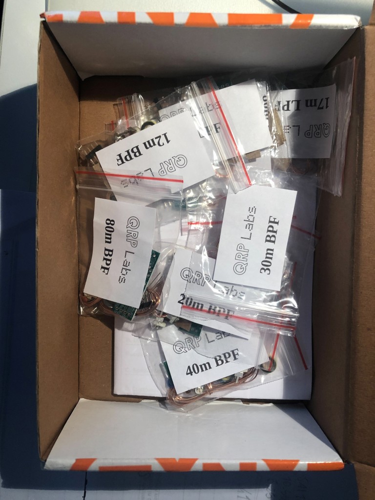
The package is well done and every kit is in its plastic bag.
Here below, I reported a pair of pictures during the unboxing.
Now let’s talk about assembly and performance.
No printed assembly instructions is provided. The pdf must be downloaded, as written on the website. It contains very good explanations and it’s quite impossible to do a wrong assembly after carefully reading it. Layout and other images help to easily find out the component positions. A table contains all the capacitors and inductors values (so number of turns) for all the bands. A clear explanation of the correct intepretation of the capacitors marking is also included.
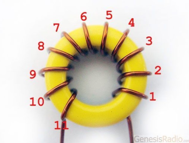
The most difficult part is the inductors winding, but some useful tips are reported by QRPLabs for a correct winding procedure and methods for scraping the enamel off by the insulated wires.
Particular care should be taken for counting the windings, because it could be confusing. Every time the wires goes to the toroid center , it’s a turn. If you want to count the windings of a finished inductor, you have to count the wires inside the the core. If you count wires in the external part, you will find one turn less and it could be very confusing! The image below helps to identify a correct method.
Up to now, I’ve built and characterized the following filters:
LPF 80meters
LPF 40meters
LPF 30meters
LPF 17meters
LPF 12meters
BPF 30meters
I didn’t finish the switch board yet, but it’s very easy compared to the filters, because there isn’t any inductor to wind.
I followed the instructions and obtained working filters at first shot! Here below the pictures of assembled LPF filters:
Here below, the pictures of BPF 30meters , the only one that I had time to build.
Particular attention should be taken for the BPF that are only two, but aAdditional small windings are added on each toroid, turning them into a transformer with primary and secondary part. These short windings form the input and output of the filter. The turns ratio is chosen to achieve the usual 50 ohm input and output impedance.
Here below a particular of the transformer:
As you can see, the primary winding is made of thicker wire, because it helps to distinguish the primary from secondary when you go to solder it on the PCB!
Primary windings has to be soldered directly to the header pins of the filter, as reported below:
I reported a useful note of QRPLabs manual, that I always follow:
“…you will certainly need to adjust the number of turns to get the filter centre frequency correct. It is easy to remove one turn. But very difficult to add one! To add one you have to solder on an additional piece of wire and things get messy. So start by winding 4 turns too many – and you can then easily remove them one by one until you hit the exact right centre frequency…”
Although this prudence, the number of turns matched exactly the instructions and no extra turn was needed.
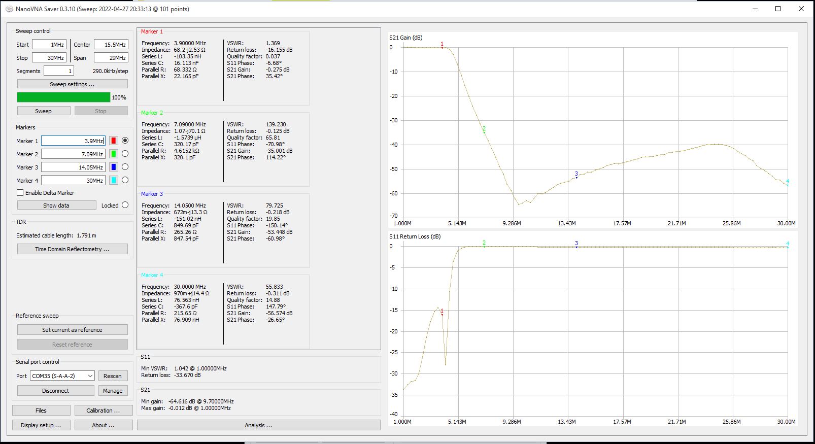
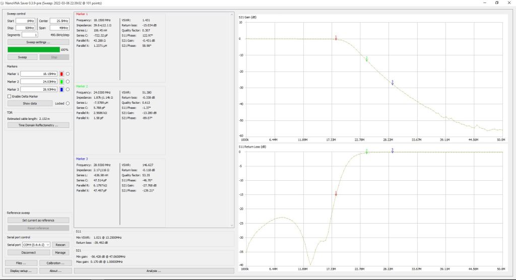
Here below, some pictures of the LPF filter measurement done with my NANOVNA are reported:
80meters LPF S21 and S11
40meters LPF S21 and S11
30meters LPF S21 and S11
17meters LPF S21 and S11
12meters LPF S21 and S11
In order to connect the VNA SMA cables to the 4pins headers of the filter, I built simple adapters, which are visible in the picture below.
Note that the ground wires shall be as short as possible, otherwise they could form loops. Initially, the filter showed a very poor isolation performance due to coupling effects between these adapters!
If you want, a PCB fixture with PCB-mounted SMA female connectors is better and more stable.
On the internet, there are nice fixture projects that are much better of my “quick&dirty” approach.
As you can see from the measurements, the in-band and out of band attenuation and roll-off are in line with the theoretical performance of a 7th order Butterworth filter.
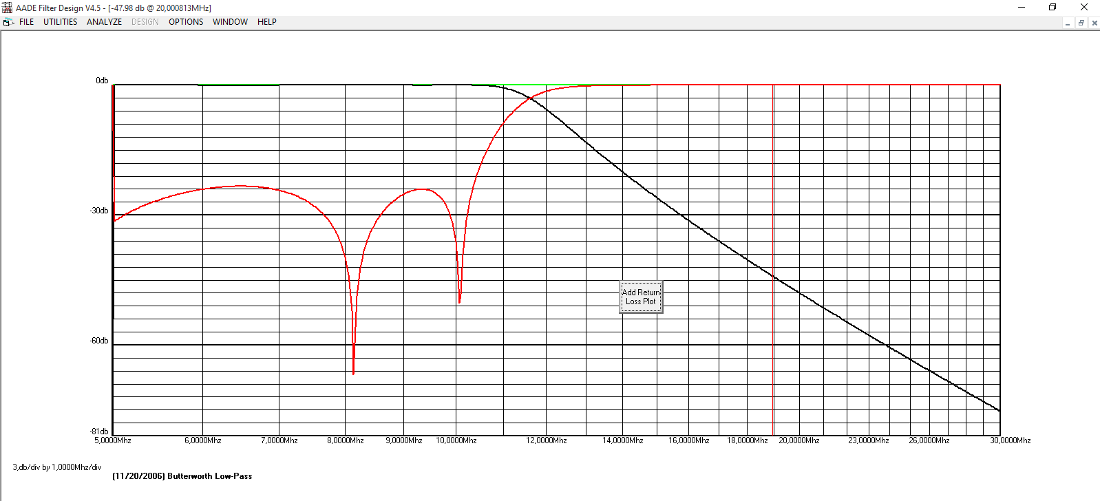
As example, I reported below the comparison between measurement and simulation of the 30meters band filter. On the top of simulation picture there is the reding of the red marker, which shows -48dB @ 20MHz, and is quite similar to the measurement (-50dB).
The VNA has a limited dynamic and can’t reach the -80dB showed by the simulation.
On 17 and 12meters filter, the cut off frequency is very near to the center band frequency (you can see the “knee” starting immediately after the marker), but it’s not a problem.
Here below, I reported the measurements of the 30meters BPF band. It has been very easy to tune it on the center frequency and no modifications on the windings have been necessary.
30meters BPF S21 and S11
30meters BPF S21 and S11 – zoomed
In the second measurement, the delta marker has been activated in order to highlight the Band at -3dB referred to the center frequency. The BandWidth is more or less 940KHz.
Before starting the assembly, I searched for reference measurements on the internet, but I couldn’t find them, so I hope the measurements can be useful to other OMs that are going to build the filters.
I will update the article when other BPF filters and the switch board will be ready and characterized!
Best 73’s
Alfredo IZ7BOJ
EDIT 16/05/2022
Once I wrote this article, I shared it on QRPLabs newsgroup.
One OM, Lex PH2LB, appreciated my work and he sent me one of his fxture kit specially designed for measuring QRPLabs filters using NanoVNA.
The fixture is available in different formats which differs for the spacing between sma connectors. The spacing allows to connect the fixture directly to the VNA withut any cable.
Moreover, Lex added SMD calibration standards on the board, which can be selected with 2,54mm jumpers. This idea has three main advantages:
makes the calibration faster
no externals short-open-load-thru standards are needed
makes the calibration much more accurate because it includes the fixture itself
The kit includes also a 3D-printed case which is open on top, and is very straight-forward to build.
I tried it and the results are very similar to my home-made fixture, but I’ll always use this fixture because it makes the measurements more reliable and repetitive. I suggest it for OMs who want to play very frequently with these filters.
Here below some pictures of my fixture with and without filter on top:
Here below, I reported the measurement that I repeated for 30meters LPF filter, just for comparison with the first, taken using my fixture. The results are very similar.
APRS (Automatic Packet Reporting System) is an amateur digital communications system that uses packet radio (usually 1200bps) to send real time tactical information like coordinates, altitude, speed, heading, text messages, alerts, announcements, bulletins and weather data on amateur radio frequencies.
APRS data are typically transmitted by mobile stations and gathered to the APRS Internet Service by Internet-Gates, which are connected to internet and have a radio interface listening packets. Usually, these stations are located on top of mountains or in places where the radio coverage is good.
If the land is vary flat and I-gates have not good coverage, sometimes the mobile stations can’t reach directly the I-gates, then digipeater (digital-repeater) stations acts like “fill-in” stations to improve the coverage, receving mobile packets and retransmitting them to I-gates.
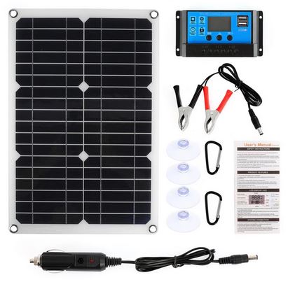
With aprspuglia group , we considered to extend the aprs coverage in my region putting a digipeater in the rural zone. Unfortunately, it’s not easy to have an electric power source, so I decided to experiment a solar digipeater keeping the cost as low as possible.
The solar kit I bought is this, from aliexpress, for about 30$.
The discharge stop voltage protects your battery from extreme discharge damage. Should your battery get heavily run down, this threshold kicks in and disconnects the load. Lead acid batteries can be damaged if deeply discharged. This of course means your digipeater is off the air until the sun recharges your battery. The equipment should be connected to the LOAD connection on the regulator to take advantage of this option.
In my case, the default Discharge stop voltage is set to 10,5Volts.
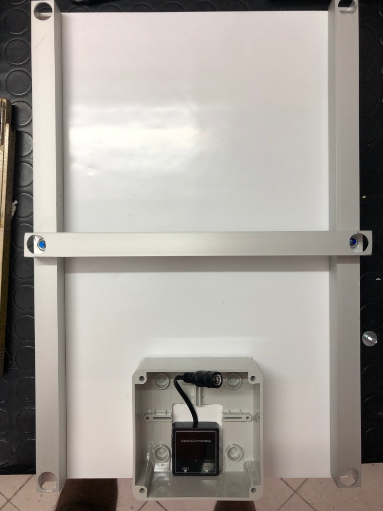
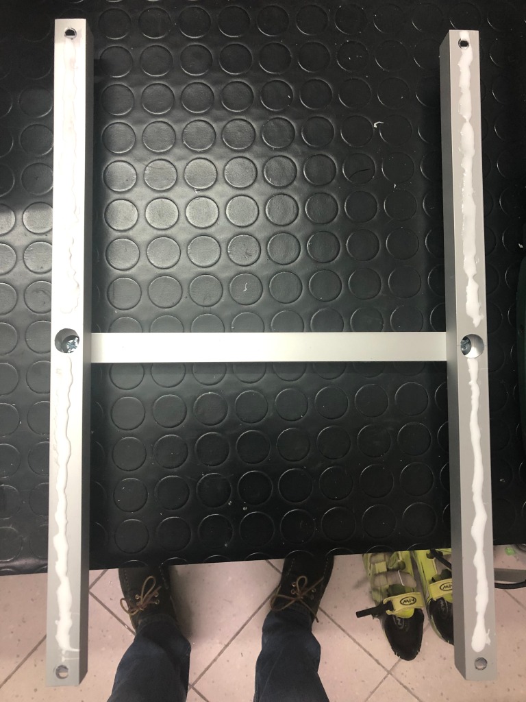
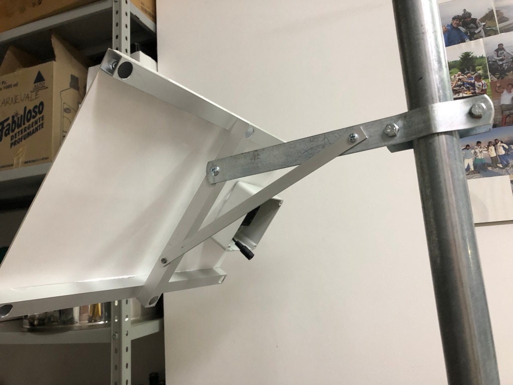
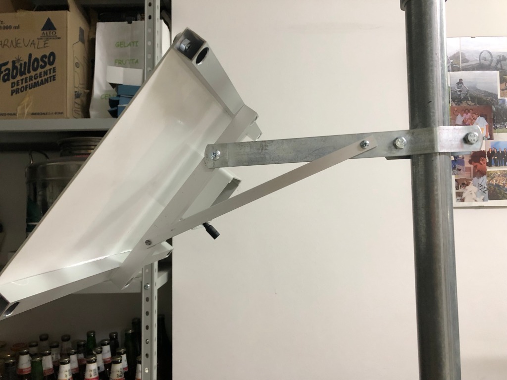
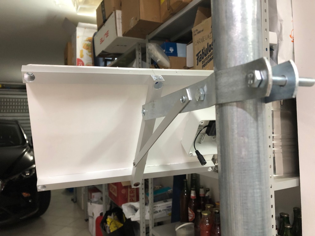
The solar panel is based on a thin plastic plate. It’s designed for camper/mobile use, so I had to build a solid support for fixing it on the pole.
With about 10€ of clamp and square aluminum profiles, I built a simple “skeleton” for the scope. The structure is mounted with some 10mm nuts and bolts. The solar panel is mounted on the structure with same bolts and with some silicon glue.
The panel is inclined by 45degrees and distant enough from the pole.
The other part wich is not designed for outdoor use is the electric connectors. As you can see from the pictures, the panel comes with a small black box with an internal regulator and two USB ports (which I don’t need). From this box, a power cable with a female jack is also available.
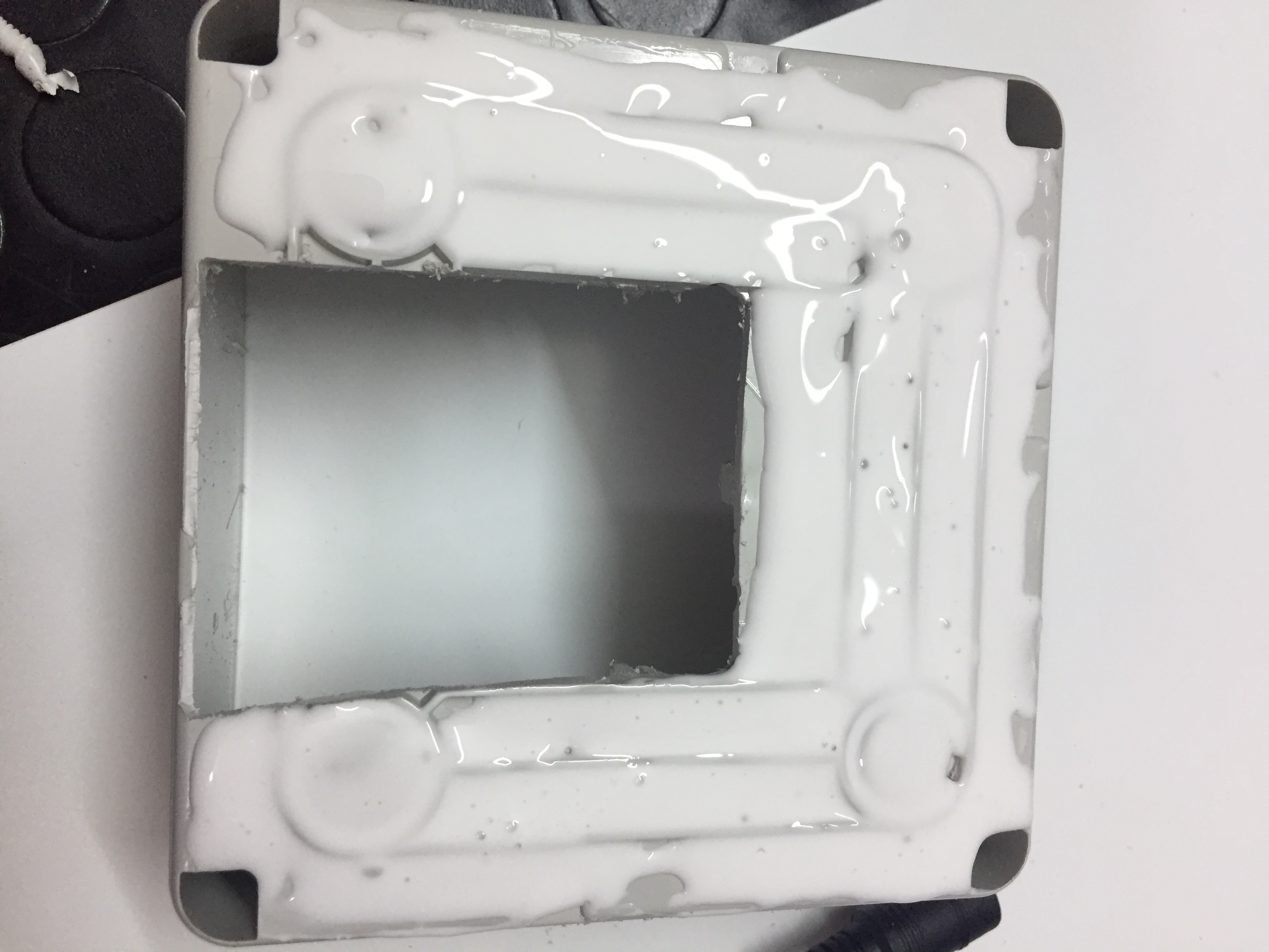
To make the panel suitable for outdoor, I had to enclose this black box inside a PVC electric box, glued to the panel. I cut away the power jack and soldered a 2x1mm cable which goes to the digipeater box.
Here below some detailed pictures.
The bluepill is powered by one of the two usb ports available on the controller, while the radio is powered directly by the 12V output of the controller.
The radio doesn’t have a dedicated power-in jack, because it’s designed to be used always with its battery pack, so I build a cable with two ring terminals that I fixed on the spring contacts dedicated to the battery pack:
I think the declared power is not realistic, but even if I consider half of the value, it shold be enough to charge a 7Ah lead acid battery. Some easy calculation of power budget demonstrate that this configuration is enough to keep the digi alive during all day, even during a cloudy day.
The radio is one of the most important part of the project.
One of the cool things about APRS is you can use almost any old VHF amateur radio to get the job done. You don’t need tone or memories as everything occurs on one frequency. Even an ancient radio from the 1980’s will work great!
A handheld radio has the benefit of being small and will generally have a much lower battery drain when idle. The downside to using an handheld transceiver is a max of about 5w output on most models, but for most of fill-in digi, this power is more than enough to reach the first i-gete.
Luigi IZ0YAY borrowed me an Intek KT-210 radio, which has an extremely low battery draw as it has no fancy features and no digital display. It uses thumbwheels to set the frequency. An added advantage to those old thumbwheel radios is they go right back on frequency if the power gets cycled.
The receivers on most handheld radios leave much to be desired when it comes to selectivity. Seems the newer the radio, the worse this got. The Intek radio has a decent receiver in it and it sinks only 65mA in receiving mode, which is great! Moreover, it must be considered that the installation site is free and far away from strong RF sources like TV/radio broadcast transmitter or repeater. The farm is lost in the country 🙂
The TNC is another core part of the digi. I chose the SQ8VPS VP-Digi, which is actually the most powerful and flexible TNC with digipeater capability at the moment, in my opinion. The power consumption is very low, as it is based on a Bluepill delvelopment board (STM32 microcontroller).
VP-Digi offers 8 configurable beacons and an APRSdigipeater, which is capable of handling 4 type n-N aliases (e. g. WIDEn-N, NYn-N) and 4 simple aliases (e. g. CITY, AREA). Moreover, the digipeater incorporates the viscous delay function know from aprx, which can reduce unnecessary traffic. There is also a posibility to filter packets by sender callsign, either in blacklist or whitelist mode. The digipeater can be freely configured, e. g. to work as regional (Wn) or fill-in (W1) digi.
The device is equipped with an USB port and two UART ports. All of them can work independently in KISS TNC, frame monitor or configuration mode. The configuration is done by simple commands using any terminal program and is stored in the embedded flash memory.
The circuitry around the bluepill is very minimal, and consist of only an audio input filter, an audio output filter + trimmer, a BJT for TX switching and a pair of led for indication of TX and carrier detection. Seen the simplicity of the circuit, I decided to assembly it on a prototype board. Here below, the picture of the final result.
I used the PWM version, but I think there isn’t any deep difference compared to the ladder version.
The Box has been the most expensive part of the project! I chose a Gewiss Box 38x30x12cm to easily accomodate all the parts and leave some free space for future needs (example: a bigger battery). Unfortunately, the GEWISS box in my case is the most expensive part of the project, but it will be continuously exposed to the sun and the rain and it is subjected to severe temperature range. It’s better to have good quality box to prevent all the electronics from deterioration and ensure durability.
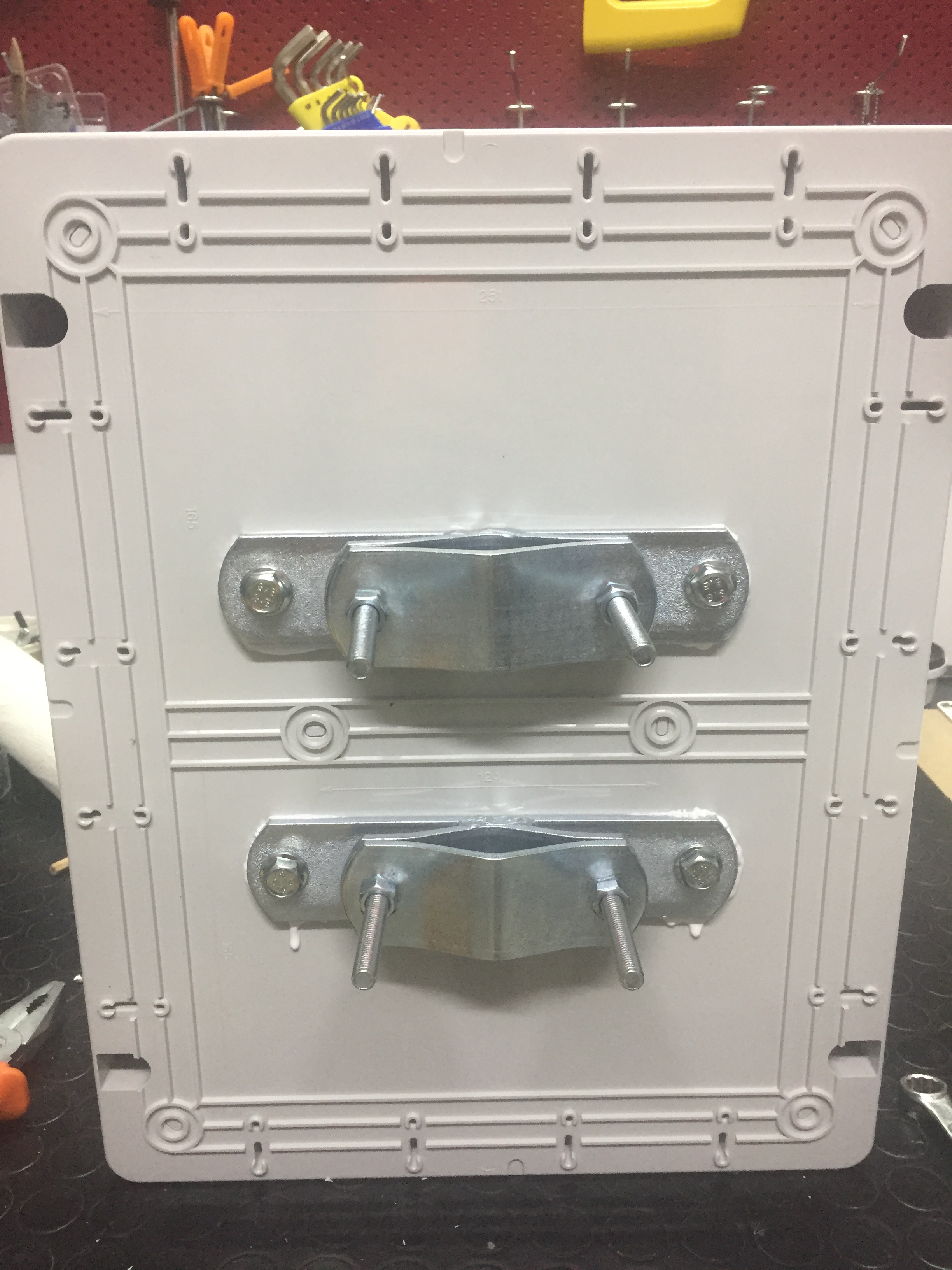
I added lower and a higer air inlets/outlets for air circulation, and I put a protection on every tube to prevent the insects from entering in the box. I used 40mm pieces of PVC electrical tube, tube to box joint and small grid, fixed to the pipe with some screws and a PVC ring obtained from the tube.
Here below, you can see how I fixed the clamps to the box. I used some silicon to seal the spaces and prevent water from entering into the box:
All the parts have been fixed inside the box by mean of self-threading screws and some home made brackets.
In the last picture I measured the current skink in rx mode and it’s only 66mA, very good.
In tx I measured more or less 600mA (out 1,5W):
The antenna and panel cables enter into the box through dedicated joint:
I configured the TNC as “fill-in digipeater” (see VP-Digi page). The beacon was set every 10minutes via WIDE1,WIDE2-1 (I can reach igate whith two hops, so the wide2-2 is unuseful)
Before the final installation, I decided to test the digipeater in my town. During the test period I never saw the tnc blocked or switched off, so the solar power is well dimensioned and the digi is stable enough for the final installation.
Moreover, I had the opportunity to test it under the rain and check the efficiency of all the sealed parts.
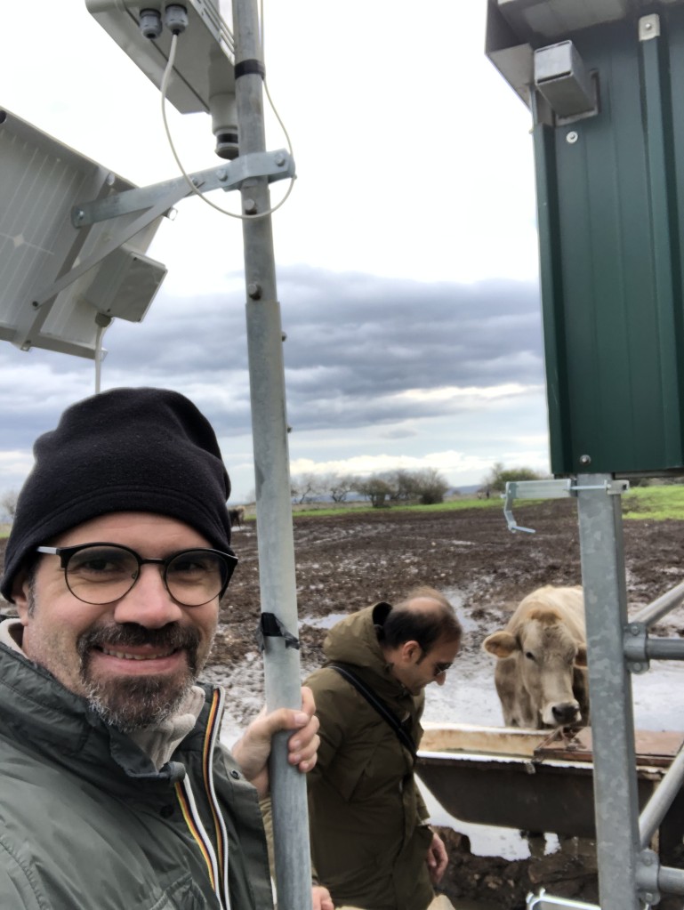
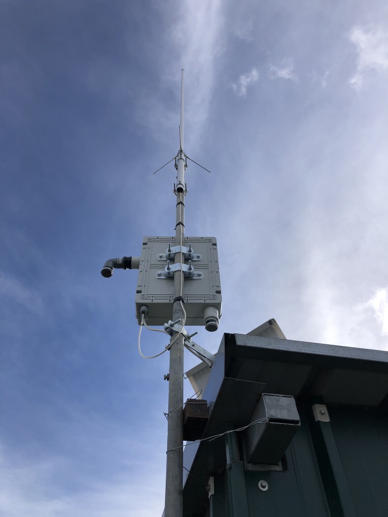
After the test phase, I started to plan the final installation. The final location is a large farm in the Murgia Mountains, at about 550m height. The pole was fixed to one of the pillars of the cows feed hut! The pole is only 4 meters high becaus it’s not possible to install bracings. The antenna installed on the top of the pole is a D-Original X-50. Here below some pictures of me, my friend IZ0YAY and the cows during the installation:
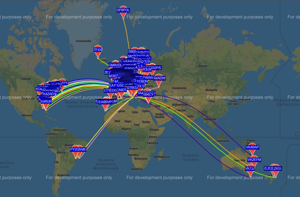
The digipeater is currently under test, but the battery duration is very good (about 2 days with no sun) and it helps the coverage in the interla Apulia area:
I hope this article could inspire other OMs for building solar applications!
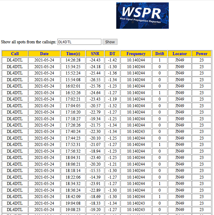
WSJT-X has a mode called wspr (weak signal propagation reporter) designed for probing potential radio propagation paths using low-power beacon-like transmissions.
WSPR beacon includes a callsign, Maidenhead grid locator, and power level using a compressed data format with strong forward error correction and narrow-band 4-FSK modulation. The protocol is effective at signal-to-noise ratios as low as –28 dB in a 2500 Hz bandwidth. Receiving stations with internet access may automatically upload reception reports to a central database.You can read more about it and see reports on the wsprnet website.
You can run WSJT-X using a regular computer and HF rig controlled via CAT in the normal way, but this ties up a lot of resources. The “poor man” WSPR can run on a raspberry pi single board computer using wsprrypi in tx and rtlsdr-wsprd using a rtlsdr usb dongle. Here below I go in detail.
RX part and web interface
The receiving part of the WSPR station relies on a RTL-SDR Dongle V2. The V2 is the only version that will work on HF band because it allows the direct-sampling. On the web, you can find a lot of article for the modification of RTLSDR V1 for direct sampling, but it’s not very easy because it’s necessary to do very small solderings. Here there is one of these articles.
The software used for WSPR decoding is the simple an powerful daemon rtldsr-wsprd. If the receiving station has an internet connection, this software also allows automatic reporting of WSPR spots on WSPRnet.
You just have to follow author’s instuction to install and run it.
NOTE: as declared on the author’s github page, the daemon can crash on Jessie OS releases and later versions, whil it runs perfectly on wheezy. If you don’t want to downgrade the release, you can just run the daemon with the “-S” (single pass) option, and it’s ok.
If you want, you can add a simple web interface which I developed to have some statistics of the received spots. My web interface is available here . The interface needs php5 and a web server installed (I use the light and poweful lighttpd)
NOTE1: if you want to run my web interface, you must use a special version of rtlsdr-wsprd modified by me. The modified version shows date and time of received spots. This feature was not present in the original version but it’s necessary for doing statistics. The modified rtlsdr-wsprd version is available here.
NOTE2:By default, the daemon doesn’t write any log, so it’s necessary to do a redirect of the standard output on a log file which will be processed by web interface for statistics. Follow exactly the instructions written on my github page for correctly run the daemon and create the log file.
Here below, I reported the main characteristics of the web interface and some screenshots.
Show number of lines in log
Show RX Load in spot/min calculated on last 20 spots
Show system status table
Show WSPRd configuration parameters in a separate table
Show last spot list, grouped by call (pivot table)
For every call, shows distance in Km and bearings in degrees with reference to receiver locator
For every call, a complete list of received spots is available clicking on “show spot details”
Possibility to make ascending or descendig sort in every column of heard stations
Possibility to show custom info editing custom.php file
You can also schedule daemon restart ad different times during the day following the propagation apertures. In this article, the procedure for setting cron daemon is well explained.
TX PART and RX/TX Switch
After the Receiving part, I decided to implement also the TX part, sharing the same antenna with a RX/TX switch.
There are a lot of solutions for implementing a WSPR beacon. The Ultimate 3S by QRPLab is one of the most elegant, but I wanted to use the same Raspberry and have a compact solution, so I decided to use this nice application: Wsprrpi, which use a GP I/O pin of the raspberry as transmit line!
The output is a square wave with plenty of harmonics (unwanted frequencies above the desired generated radio frequencies) that pollute the spectrum if you connect the RPi output directly to the antenna. The solution is to use a low pass filter between the raspberry and the antenna. The maximum output using Wsprrpi is about 10dBm (about 10mWatts). A lot of OMs use wsprrpi with a filter and no amplifier with good results; anyway a little more power would be better, so I decided also to build a Power Amplifier.
Before starting with the PA, I had to find a solution for the RX/TX switch. The frequencies and the tx power are not too high and a normal electro-mechanic relay is enough for that scope, but the problem is to find a signal for the commutation. The Wsprrpi is an open-source application, so I studied the code and also the Broadcom BCM2837 datasheet for finding the proper registers to configure another GPIO as output at set it high only during transmission.
In few hours (I’m not a professional programmer) I found the solution and successfully tested !
The modified version of Wsprrpi is available on my github and uses GPIO5 as tx switch line (high during TX).
Here Below, there is the complete block diagram of the WSPR station:
POWER AMPLIFIER
There are a lot of QRP power amplifiers that can be used for this scope, but the most interesting for me is the VK3PE project, based on Power Mosfet RD16HHF1 , suitable for Ultimate 3S WSPR beacon.
I removed the input attenuator because the Ultimater 3S gives 180mWatt, while raspberry only 20.
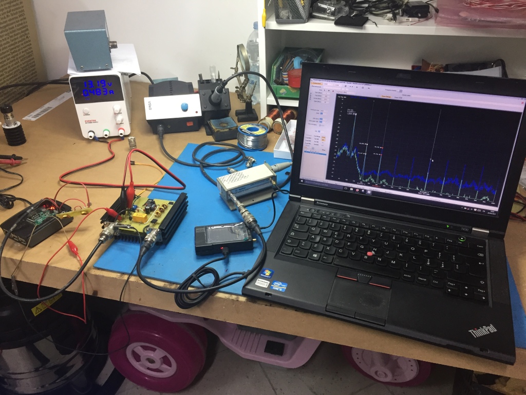
I decided to build a first prototype of the RF part, omitting the 12V switch (later I will explain why), very quickly just to have test it with the raspberry output. See picture below 🙂
The first results were good although the very bad assembly, so I decided to go ahead with a more “engineered” and stable version.
Note: during this first test, I only monitored the output with the oscilloscope and a power meter. I ordered a TinySA spectrum analyzer, but I didn’t get it in time for the test.
Since I had to use an electro-mechanical for the RX/TX switch, I decided to use a Doble Pole – Double Throw switch with the +12V on one channel and RF on the other (see block diagram of previous paragraph).
As described in the schematic notes, the binocular transformer is winded with a couple of insulated wires because this solution gives more power respect to the coax winding.
Here below some pictures taken during the assembly of the PA inside the chassis (dissipator) of an old CB amplifier, reusing the existing PL female connectors.
Before starting to solder the component, I cut the prototype board support tobe fitted inside the PA box. Then I drilled M3 holes into through PCB and into the power dissipator, and threaded these ones with my threading kit.
The power mosfet is also fixed on the dissipator using a M3 screw and thermal paste.
Note: most of the holes were used for the old CB amplifier and not for my PA.
As front panel, I cut a small piece of copper PCB and drilled to holes for the 3mm TX led and the ON/OFF Switch:
On the rear, you can see the female SMA connector dedicated to the RX output. I used a small SMA-SMA pigtail for the connection to RTL-SDR input.
Here there are some pictures of the inside PCB.
The binocular ferrite is anchored to the PCB by a cable-tie wrap.
Shielded cables are all RG174 (it should be better to use teflon insulated coax).
I also added a ferrite choke on the input power cable and winded two turns of cable around it just to be sure to block possible conducted emissions.
FILTERING
This has been the most tricky part of the project, because the Raspberry output is a square wave and it’s not good to put a squarewave onto the air!
The VK3PE project has a Low-Pass filter on the output, but not on the input, because an LPF is already implemented in the Ultimate 3S board and the input is clean enough to be amplified.
If the input LPF filter is not used, the output is full of harmonics up to 200MHz and not usable. Then I built another LPF filter and put it on the input, and the output becomes more clean.
Here below, I took two measurements made with TinySA and a 40dB filter on its input:
The 2nd and 3rd armonic are still present but at about -55dBc so they are acceptable.
Since the RTL-SDR dongle doesn’t have a band pass filter on its input. It works in direct sampling and so aliasing will occur. The RTL-SDR ADC samples at 28.8 MHz, thus you may see mirrors of strong signals from 0 – 14.4 MHz while tuning to 14.4 – 28.8 MHz and the other way around as well. To remove these images you need to use a low pass filter for 0 – 14.4 MHz, and a high pass filter for 14.4 – 28.8 MHz, or simply filter your band of interest.
For this reason, I decide to share the LPF filter of the PA with the receiving path, so I put the LPF between the RX/TX switch and the antenna (see PA block diagram).
After some research on the internet, I decided to use G3RJV’s sheet from GQRP (Chebychev, 7th order) and selected the 30m filter.
The inductors are winded on T37-6 toroids. The characteristics can be found on www.toroids.info.
The filter is arranged on a separate small pcb with standard 2,54mm strip contact. In this way, I can easily change the proper filter if I want to change the operating band. An automatic filter bank commanded by GPIO pins of raspberry is already in my mind and I’ll try to build during some nights 🙂
Here below, the frequency response obtained by nanoVNA is reported below. Consider that with some additional tuning, the insertion loss can be better.
LABORATORY TESTS
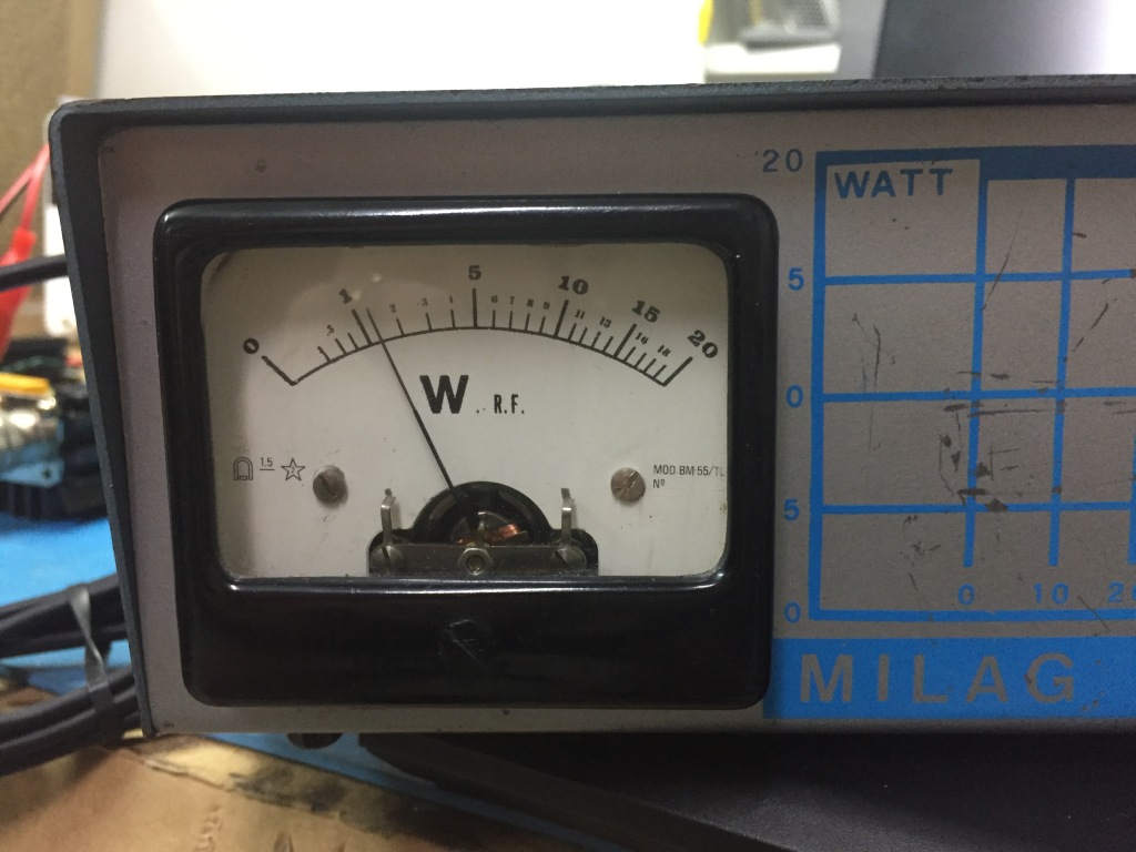
Before operate the PA, the bias trimmer must be adjusted for the minimum voltage. Then the PA can be powered and fed with a test signal (from a raspberry or other lab source, if you have), then the TX input pin can be driven high. At this point, the bias can be slowly adjusted for 650mA (600 is suggested for the Mosfet, but the other 50mA are sinked by the relay and the led).
The output power shall be about 1,5Watts (more than enough for WSPR operations) and the output spectrum shall be like the picture showed in the “Filtering” paragraph.
I left the PA continuously in TX for about 5 minutes to observe the stability and the mosfet temperature.
It should be considered that a WSPR beacon will take about 110 seconds to be transmitted, but the transmission rate should not exceed once every 10 minuts to avoid frequency saturation.
I monitored the temperature with an infrared meter directly on the mosfet body (which have a good IR emissivity) and it was about only 36 degrees, thanks to the oversized heat dissipator. You can also use a smaller dissipator.
Well, about 20 years ago, when I lived in a building with a small roof and I couldn’t install log wire antennas, I decided to build a coax trap dipole for HF bands, based on a project reported in a well known italiank book named “Costruiamo le Antenne Filari” (let’s build wire antenna) by Nerio Neri I4NE and Rinaldo Briatta I1UW.
I was attending high school and I was at the firs experience with my hamradio activity, so I didn’t have a grid dip meter, which was highly reccomended also by the authors to verfy the exact trap resonance.
I wanted to build this antenna anyway, so I tried to replicate exactly the project respecting every measure with millimetric precision, with the hope to do only little adjustment on the dipole arms lenght. But everyone who have worked with RF, knows that in practice it’s very difficult to do a trap dipole with a SWR meter only!
I built the antenna using 2,5mmq electric cable, a 1:1 balun, and built the traps using 40mm diameter plastic pipes for hydraulic systems and RG58 cable.
The coax traps were assembled in the classic configuration of the picture below:
The construction details of the trap were not published for copyright reasons.
Since the plastic pipe was not too strong, I decided to insert a small piece of 16mm pvc pipe inside the trap, and to fix the dipole to this pipe, avoiding the stress or break of the trap (see pictures later in the article).
I installed the dipole on top of a 10m pole and kept 120 degrees as arms aperture. As usual, with trap dipole the tuning should start from the higher band, which corresponds to the lenght between the traps closest to the feeding point, and then go on to the lower bands. I spent a lot of time searching for the first resonance, without any success. With much disappointment, I uninstalled the dipole and left it in a bag in my garage.
When I moved to my actual home, I went in the old garage and… I saw this old project and I remembered how much time I spent trying to let it work! But in the meantime I gained theoretical and practical experience. I don’t have a grid dip meter, but I have a NanoVNA, sto…I decided to begin another battle with this dipole!
I mad some serarch on the internet and I decided to try the following setup for searching the trap resonance frequency:
The coax trap act as parallel resonance circuit, so it looks like an open circuit at resonance frequency, while its impedance decreases at other frequencies. If the VNA channel is loaded on a 50 Ohm load and the trap is connected in parallel to this load, the return loss should show a minimum (optimal) at resonance frequency.
I did the setup as reported in the figure, with SMA to BNC transition, a BNC “T” connector and a BNC 50Ohm load. I soldered the trap terminal to a BNC male connector, and I put this connector to the free terminal of the “T” connector.
I measured all the trap resonance and I immediately understood why the dipole was not working. The 24MHz trap was resonating at about 28MHz!! All the other traps where resonating quite near the expected frequencies, but the 24MHz was completely wrong.
After different tests, I came to the conclusion that I misunderstood (or it was not clear in the book) how to wrap the trap. The plastic pipe lenght is actually too long compared to the coil, if it’s wrapped with no spacing between the turns. So I gradually started to add space between the turns and the resonance started to decrease rapidly. At the end, I reached 24MHz with all the turns spaced to the entire plastic tube, as shown below.
Then I slightly tuned all the other traps, adding some more spacing between turns and fixing the trap with plastic tape at the end. For the 24MHz trap, I decided to add some bi-component epossidic glue for fixing the turns, because the spacing was critical.
I was happy and almost sure to have found the reason the missing resonance when I was a pretty new OM, so I installed the new dipole and started to analize it with my VNA.
As soon as I did the first scan 0-30MHz with my VNA, I saw the first resonance at 24MHz! I just shortened some cm every arm, because I added some centimeters (it’s easy to cut, but not so easy to add lenght…). I was very happy for this first comfroting result which I never had during first experiments, and this told me that I was on the right way because the traps were really “isolating” the arms after the traps themselves.
Although I respected the lenght declared on my book, the resonance at 18MHz was too high, so I had to extend the wires between the 1st and the 2nd trap in order to move the resonance in the range 18.098-18.118MHz.
I had to spend a lot of time an patience to tune and optimize all the resonances, but at the end, I got good VSWR an all the bands except 40meters, on which I never get less than 1.8:1 . I tried to slightly change the spacing between the turns of the trap, but I never got values better than 1.8:1.
Here below, I attach all the measurements done with my NanoVNA on all the design bands.
In the center of the grpahs, there is a windows which shows the results of the bandwidth analysis.
Another behaviour that can be observed, is that the bandwidth drops with frequency. This probabily happens because at lower bands, the RF pass through more traps, and the “Q” factor of the traps affects the dipole bandwidth.
Here below, some picture attached.
In the picture below, I reported the original project lenghts and my experimental lenghts written by hand.
I also write some conclusions here below:
A 1:1 balun is always advisable. I used a commercial ferrite balun.
The project is quite “time-consuming” and need a lot of patience for the tuning. If you have not enough time and you need something “plug&play”, you should be better to buy a commercial trap dipole.
Considering the previuous point, I understand why the multiband trap dipole are quite expensive compared to the material costs 🙂
Always leave more wire length than the project. I suggest 30cm minimum. It’s easy to cut but difficult to add wire (I had to solder the wire and cover the soldering joint with heat-shrink tube)
During the tuning, always care about the simmetry between the lenght of the two arms
Last but not the least: the resonance of the traps shall be verified in lab before dipole installation!
This tiny device measures everything that an OM needs for his experiments and there is a ton of help on the NanoVNA forums and YouTube.
I got a lot of controversial feedbacks on the instrument, especially when used at frequency higher that UHF (theoretically the instrument reaches 3GHz..) so I decided to do a simple test with a 2 ports measurement.
Please note that the following tests don’t claim to be a complete characterization of NanoVNA. I simply write some results after some simple test.
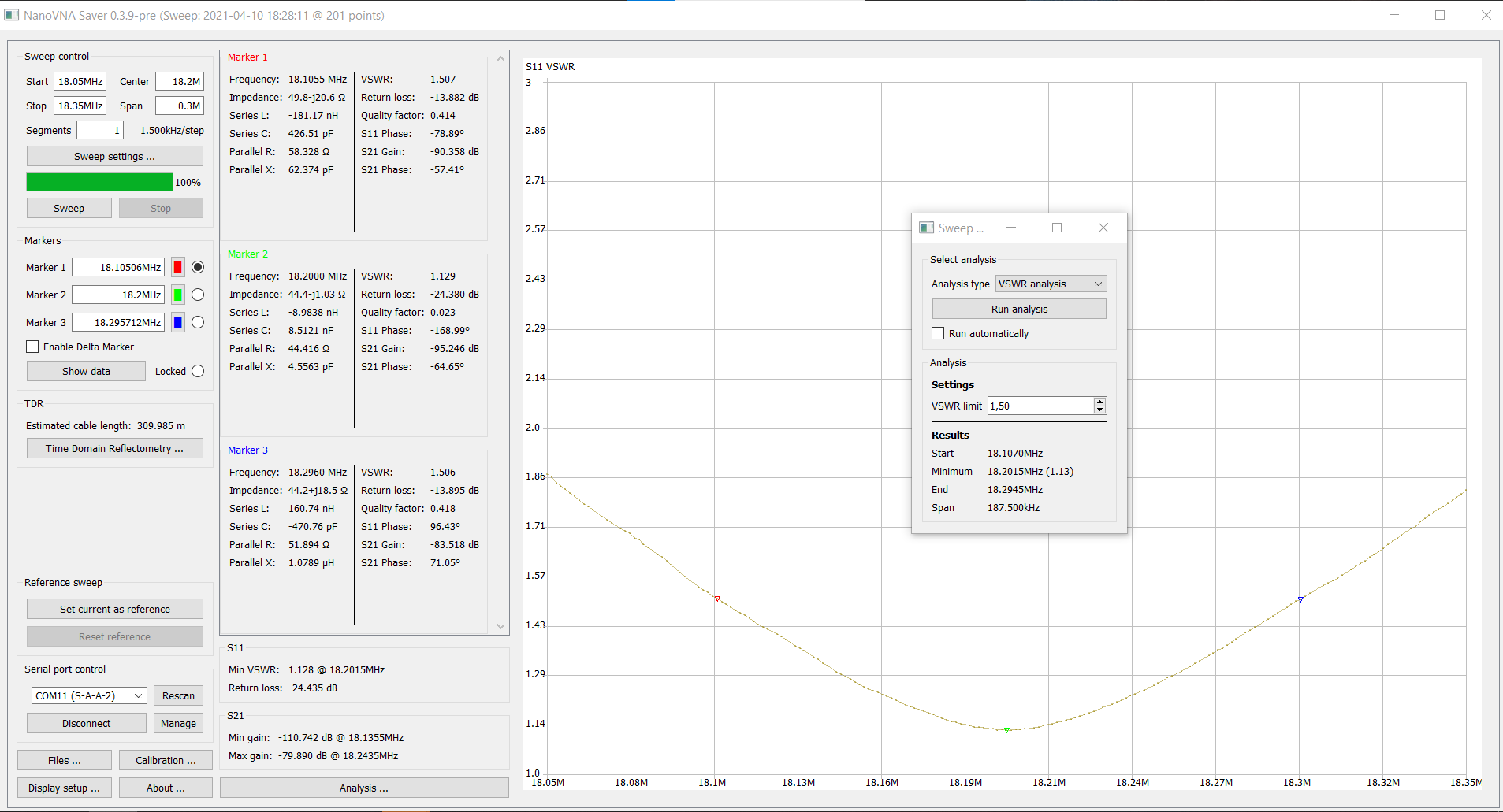
I accurately calibrated the VNA with the calibration kit in bundle.
Important Note: As suggested by NanoVNASaver during the guided calibration procedure, it’s necessary to calibrate the instrument in “stand alone” mode and store the results in one internal memories (I used “Save 0”), for better results! If I skip this step, the S21 calibration becomes really bad at higher frequencies (about 3-4 dB instead of 0dB with the through connection)! I don’t understand very well why this happens, but at the end it’s mandatory to follow the suggestion of calibration assistant.
After the verification of the S21 calibration with the SMA through connector (flat line around 0dB), I started to measure the filter with NanoVNASaver.
With NanoVNASaver it’s possible to export the graph in S2P csv file. This file is in “touchstone” format and data are stored as Real and Imaginary part for every S parameter. I imported this file in excel and then calculated the S21 in dB with the well known formula 20*log[sqrt(Re^2+Im^2)] and I easily got a result comparable to the Nooelec files.
I set the NanoVNA for 1000 points sweep, while the Nooelec includes only 600 points, but Excel can plot different series on the same graph although the “X” axis are different.
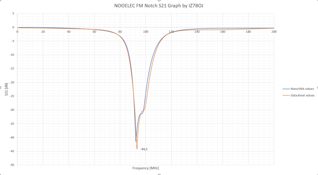
The result from DC to 200MHz is here below:
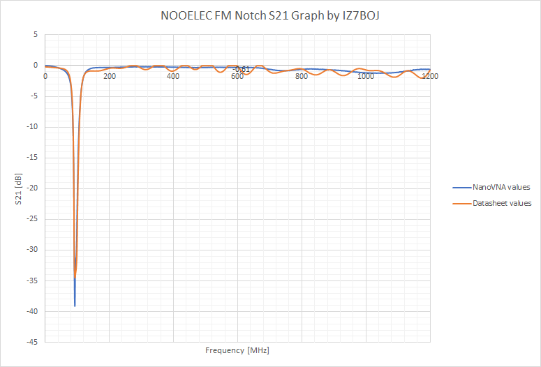
Here below, the results from 0 to 1200MHz, plotted in the same way:
It’s not too bad, considering that the Nooelec measurement is not taken on my filter and one specimen can different from other due to component tolerances. Moreover, as previously explained , the frequency resolution is different between the plots and this could giustify the deeper “hole” in the plot.
In the second figure, a ripple is present in the NOOELEC plot at higher frequencies, so I don’t know if their VNA is properly calibrated.
I’m going to do some other tests up to 3GHz. For the moment, I hope these results could be helpful to those are going to buy ad NanoVNA or a NOOELEC Filter.
I wanted to build a lightweight yagi for portable operation with my SATNOGS Az/El rotator. I surfed on the web and I found the reference site for yagi builders: DK7ZB. In the 2m/70cm-Yagis ultralight session, I found a lot of pictures of very interesting home-made yagis. I discovered that some pieces like central dipole insulator and elements supports are available on Tino’s Funkshop online store (former NUXOCOM.de) and I also discovered that, besides single yagi parts, also complete antenna kits are available.
The material for lightweight yagis is very common, so I tried to compare the price of the Tino’s Kit for 2m/70cm 13 elements Lightweight Yagi kit with the price of the same parts available on my local or online shops. I made a Bill of Material in excel with prices and… the Kit wins! Moreover, I would spent much less time for collecting all the parts and I would have the custom central dipole insulator, which is the most difficult part in my opinion.
I ordered the kit for only 21,49€ (!), payed with PayPal and I got it in a week . The shipment expenses outside Germany are about 15€ and the courier is DHL. In case of small purchases, the shipment is not negligible. Anyway, The packaging was perfect and tha materials inside were unharmed. The kit content is shown below:
The kit is composed by the following parts:
PVC tubes for Boom, 20mm diameter
20mm PVC Clips, for elements support
3,2mm aluminum rods, for all elements except radiator
4mm aliminum rod, for radiator element
7.5 x 4.5 x 4 cm PVC box, for feeding point
N panel connector
Small piece of 16mm PVC tube for RF choke
Small Piece of RG188 cable for RF choke
2 metal lugs to be soldered to RG188
brass terminal strip with screws, 4mm inner diameter
All needed screws
Detailed instructions and datasheet
I’m going to describe main steps for building the antenna
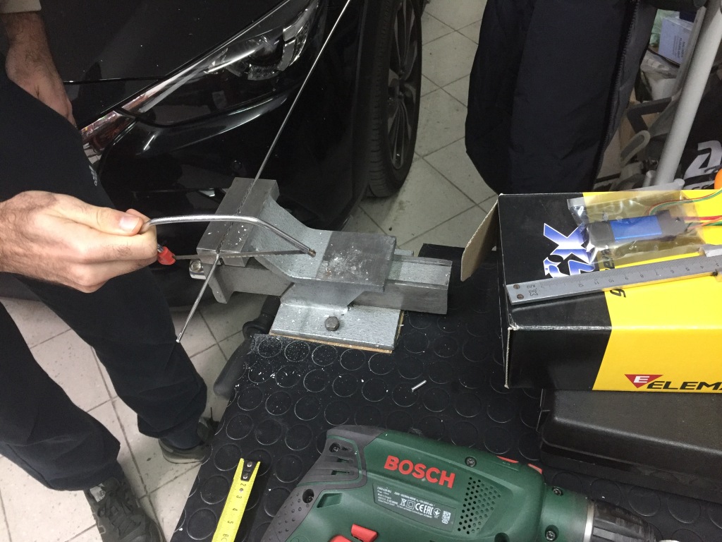
Cut all the elements to the lenght indicated on the datasheet. Be precise at mm! After the cut, remove the aluminum burrs using a flat lime.
Since the VHF reflector is longer than 1meter and the aluminum rods are 1m long, it’s necessary to lengthen it with one rest of piece from other reflectors and using the mammut connector, as the image below:
2. Drill holes in the PVC clips using 3,2mm tip. You can also try to use a 3mm tip and enlarge the hole moving slighthly the drill back and forth. In any case, you can use some glue if the element will not stay in its position. I used a stand for the drill, in order to to perpendicular holes. Anyway, don’t care if you don’t have a stand and the holes are not perfectly parallel to the clip edge, you can do small rotation once the clip is mounted on the boom.
3. Let’s insert the elements in the clamps and mark the element name in order to make the positioning easier.
4. Now, let’s proceed to the most particular part, the feeding point of the dipole.
First of all, the central hole of the insulator shall be enlarged with a 4mm tip:
Then, 2 holes of 4mm diameter shall be made on the sides of the PVC box. The caliper helped me for calculating the exact position. The, the two half dipoles can be pushed inside the insulator, passing through the box walls:
4. Now, two holes of 2,5mm diameter shall be made in the aluminum, using the insulator as guide. Don’t push too much the drill, otherwise the insulator will be ruined!
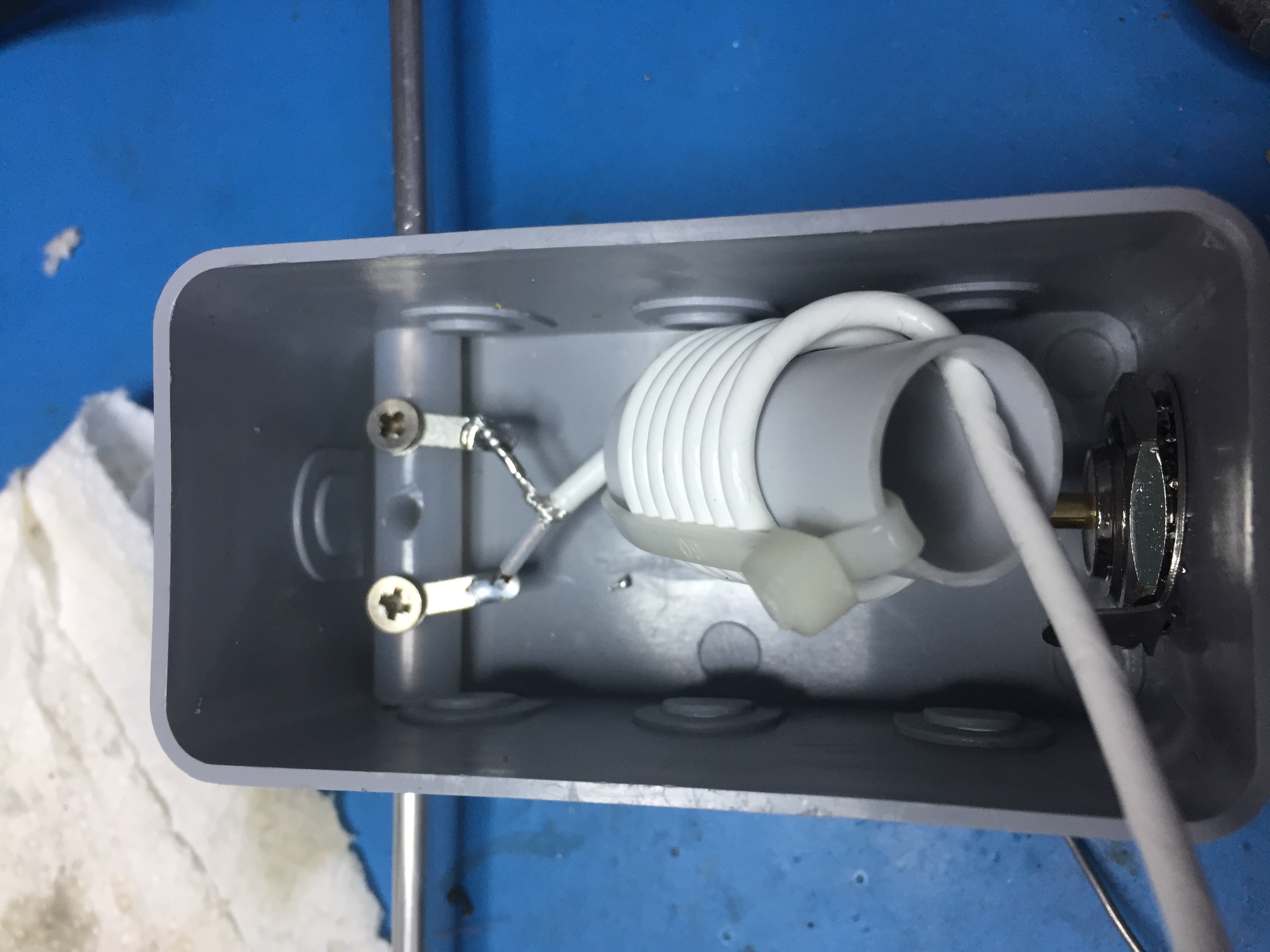
Now, the two metal lugs can be fixed on the dipole halves by two 2,9x9mm screws:
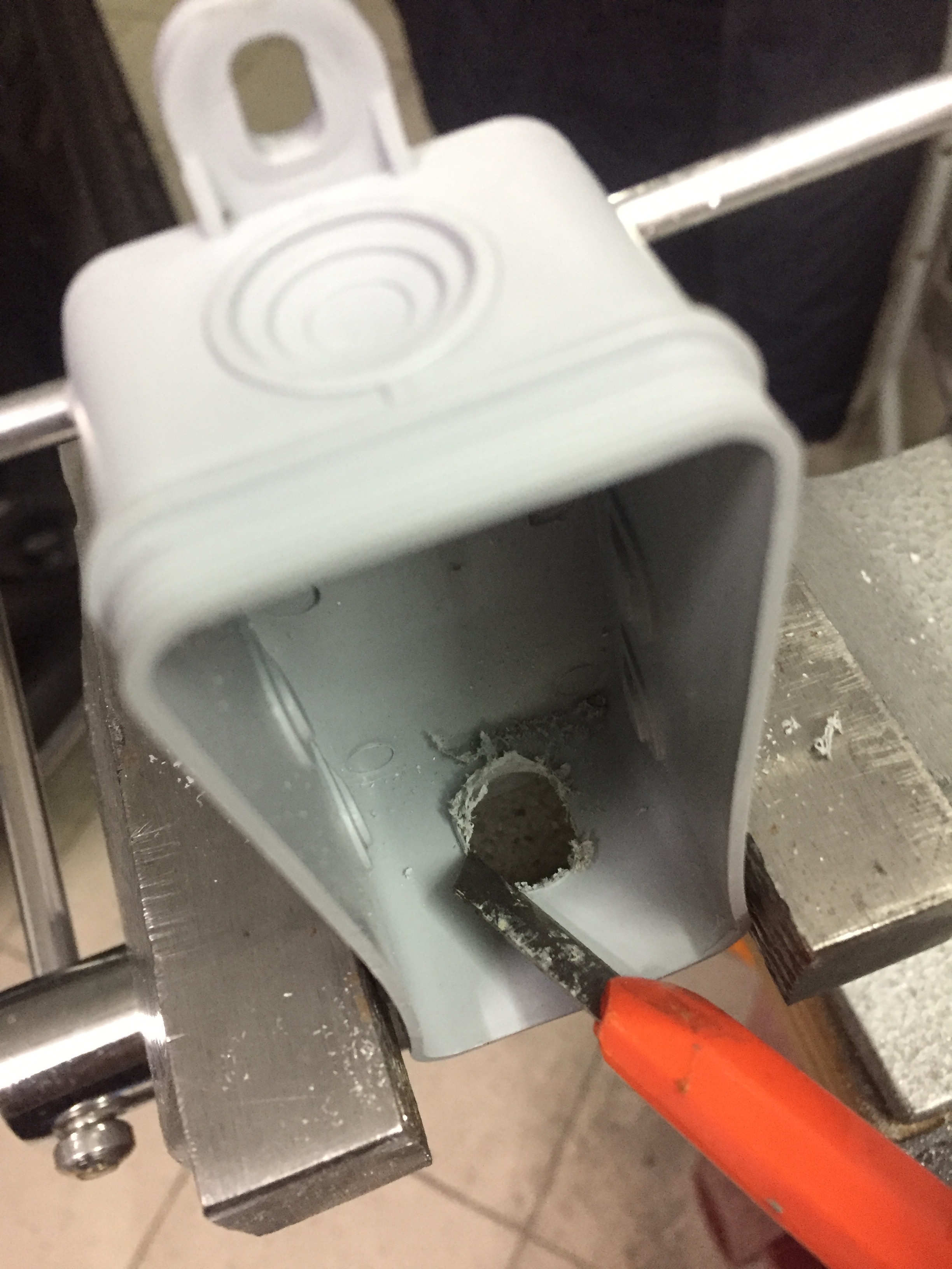
5. Now le’ts install the N socket connector to the other short side of the box. The connector has two flat notches in the threaded part in order to avoid rotations, so I suggest to drill a 11mm hole first, than work with patience and files (flat and round) as long as the connector fits inside the hole.
6. Now it’s the time to build the RF choke. Let’s drill two 3mm holes in the 16mm PVC tube and do at least 5 windings of coax cable. In my case, I did 6 windings.
Now we have to solder the coax on the dipole lugs and to the N connector. Be patient, because there is not too space inside the box. Nose pliers help in this case. Keep the unshielded part of the cable as short as possible. No matter which conductor you solder on left and right side.
7. Now let’s mark the position of the elements on the boom
This is the final result. The antenna is laying on the table of my Lunchroom. Not too bad 🙂
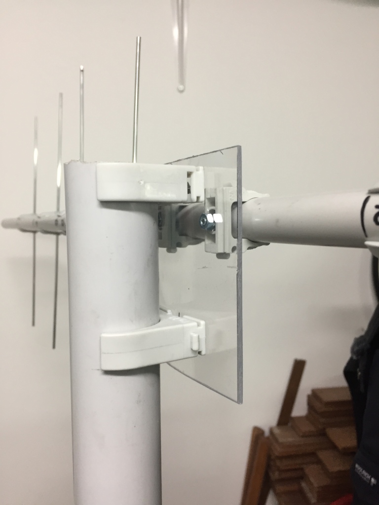
Since the antenna has an insulating boom, also the supporting tube should be not conductive. I had a 40mm PVC pipe in my garage, so I built this simple 90 degrees support using a small piece of plexiglass, a couple of clips for 20mm tube and a couple of clips for 40mm tube:
Then I started the first tests of my antenna. I put the antenna in my garage (it would be better to work in open space..):
The first check, using default design dimensions, showed this situation for 2m and 70cm:
As you can see, it’s not too worth for the beginning, so it means that I did a good job.
For both bands, I placed three markers: red at the beginning of ham band, green at center and blue at the end. The span is greater than the usable bandwidth in order to have a better understanding of the antenna behaviour.
As suggested on the manual, I started to tune the VHF resonance, so I started to cut 2 or 3 mm at time on both ends of VHF radiator. The resonance vary quickly with the lenghts, so be patient and don’t exceed with the cut lenghts!
At the end of the tuning, I got 980mm. The starting design lenghts was 995, so I cut 15mm. The resonance is shown below. It’s not perfectly centered at 145, but the SWR is <1:1.3 across the whole 2m band, so it’s ok for me:
As suggested by Nuxocom, I started to move the Open Sleeve radiator of 70cm for UHF tuning. The open sleeve is the passive element which is very near to the 2m radiator, and it’s a passively coupled radiator excited by the 2m radiator. I didn’t lower the resonance as much as I wanted in this way, so I started to cut the open sleeve (it’s allowed by nuxocom). At the end of tuning, the open sleeve was 320mm. The desing length was 329mm. The final situation is shown below:
The VSWR response is very flat and it’s <1.3:1 anyway. Good!
Now I’m waiting for real tests/comparison in open air, but i have to wait for better weather condition to go on my roof.
Concluding, the kit is highly suggested for OMs that have a minimum of manual skills and like to build antennas, but at the same time don’t have too much time for collecting material and want to start from a well tested configuration in order to have guarantee of success!
The kit is very complete and nothing else is necessary to build the antenna. The quality of the materials is very high and the price is very cheap compared to local shops.
Building instrunctions are also very detailed and easy to understand.
Everyone can customize the antenna and follow different solutions, but the suggestions, in my opinion, are the best way for good and quick results.
The only modification that I would consider, is to replace the steel screw and nut at the center of the dipole insulator (not visible in the previous pictures) with a nylon equivalent, since the screw is very near to the radiator parts (the center gap is only 10mm).
I didn’t have a 4mm nylon screw during the assembly, otherwise I would have changed it.
I hope this could help next OMs that want to build a twinband yagi and would consider a kit.